You can find the Jupyter Notebook for this project here. For access to the .csv file, which was too large to upload to Github, use the Contact form on my website.
Beep… Boop… Beep…
Part of my OKCupid Capstone Project was to utilize machine learning to create a classification model. As a linguist, my mind immediately went to Naive Bayes classification– does the way we speak about ourselves, our relationships, and the world around us give away who we are?
During the early days of data cleaning, my shower thoughts consumed me. Do I break down the data by education? Vocabulary and spelling could differ by how much time we’ve spent in school. By race? I’m sure that oppression has an effect on how people speak about the world around them, but I’m not the person to provide expert insights into race. I could do age or gender… What about sexuality? I mean, sexuality has been one of my loves since well before I started attending conferences like the Woodhull Sexual Freedom Summit and Catalyst Con, or teaching adults about sex and sexuality on the side. I finally had a goal for a project and I called it– wait for it–
The Gaydar.
TL;DR: The Gaydar used Naive Bayes and Random Forests to categorize users as straight or queer with an accuracy score of 94.5%. I was able to replicate the experiment on a small sample of current profiles with 100% accuracy.
Cleaning the Data:
The Beginning
The OKCupid data provided included 59,946 profiles that were active between June, 2011 and July, 2012. Most values were strings, which was exactly what I didn’t want for my model.
Columns like status, smokes, sex, job, education, drugs, drinks, diet, and body were easy: I could just set a dictionary and create a new column by mapping the values from the old column to the dictionary.
status_map = {'unknown': -1, 'single': 1, 'available': 2,
              'seeing someone': 3, 'married': 4}
df['status_code'] = df['status'].map(status_map)
The speaks column wasn’t terrible, either. I had considered breaking it down by language, but decided it would be more efficient to just count the number of languages spoken by each user. Thankfully, OKCupid put commas between selections. There were some users who chose not to complete this field, and we can safely assume that they are fluent in at least one language. I chose to fill their data with a placeholder.
df['speaks'] = df['speaks'].fillna('unknown')
df['languages_spoken'] = df.apply(lambda x: x['speaks'.count(',')+1, axis=1)
The religion, sign, kids, and pets columns were a little more complex. I wanted to know each user’s main choice for each field, but also what qualifiers they used to describe that choice. By performing a check to see if a qualifier was present, then performing a string split, I was able to create two columns describing my data.
def get_religion(religion_str):
    religion_map = {'unknown': -1, 'atheism': 0,'agnosticism': 1,
                   'christianity': 2, 'catholicism': 3, 'judaism': 4,
                    'buddhism': 5, 'hinduism': 6, 'islam': 7,
                   'other': 8}
    if ' ' not in religion_str:
        religion = religion_str
    else:
        religion = religion_str.split(' ',1)[0]
    return religion_map[religion]
def get_religion_serious(religion_str):
    serious_map = {'and laughing about it': 0,
                   'but not too serious about it': 1,
                   'and somewhat serious about it': 2,
                   'and very serious about it': 3}
    if ' ' not in religion_str:
        serious_code = -1
    else:
        serious = religion_str.split(' ',1)[1]
        serious_code = serious_map[serious]
    return serious_code
df['religion'] = df['religion'].fillna('unknown')
df['religion_code'] = df['religion'].apply(get_religion)
df['religion_serious'] = df['religion'].apply(get_religion_serious)
The ethnicity column was similar to the languages column, in that each value was a string of entries, separated by commas. However, I didn’t just want to know how many races the user input. I wanted specifics. This was slightly more effort. I first had to check the unique values for the ethnicity column, then I browsed through those values to see what options OKCupid gave to their users for race. Once I knew what I was working with, I created a column for each race, giving the user a 1 if they listed that race and a 0 if they didn’t.
I was also interested to see how many users were multiracial, so I created an additional column to display 1 if the sum of the user’s ethnicities exceeded 1.
df['ethnicity'] = df['ethnicity'].fillna('unknown')
df['ethnicity_white'] = df.apply(lambda x: 1 if 'white' in x['ethnicity'] else 0, axis=1)
df['ethnicity_black'] = df.apply(lambda x: 1 if 'black' in x['ethnicity'] else 0, axis=1)
df['ethnicity_other'] = df.apply(lambda x: 1 if 'other' in x['ethnicity'] else 0, axis=1)
df['ethnicity_hispanic'] = df.apply(lambda x: 1 if 'hispanic / latin' in x['ethnicity'] else 0, axis=1)
df['ethnicity_pacific_islander'] = df.apply(lambda x: 1 if 'pacific islander' in x['ethnicity'] else 0, axis=1)
df['ethnicity_native_american'] = df.apply(lambda x: 1 if 'native american' in x['ethnicity'] else 0, axis=1)
df['ethnicity_middle_eastern'] = df.apply(lambda x: 1 if 'middle eastern' in x['ethnicity'] else 0, axis=1)
df['ethnicity_indian'] = df.apply(lambda x: 1 if 'indian' in x['ethnicity'] else 0, axis=1)
df['ethnicity_asian'] = df.apply(lambda x: 1 if 'asian' in x['ethnicity'] else 0, axis=1)
df['multiracial'] = df.apply(lambda x: 1 if (x['ethnicity_white'] + x['ethnicity_black'] +
                             x['ethnicity_other'] + x['ethnicity_hispanic'] +
                             x['ethnicity_pacific_islander'] +
                             x['ethnicity_native_american'] +
                             x['ethnicity_middle_eastern'] + x['ethnicity_indian'] +
                             x['ethnicity_asian'])>1 else 0, axis=1)
The Essays
The essay questions at the time of data collection were as follows:
- My self-summary
- What I’m doing with my life
- I’m really good at
- The first thing people notice about me
- Favorite books, movies, shows, music, and food
- Six things I could never do without
- I spend a lot of time thinking about
- On a typical Friday night I am
- The most private thing I’m willing to admit
- You should message me if
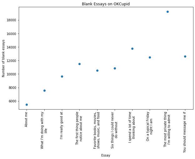
Almost everyone filled out the first essay prompt, but they ran out of steam as they answered more. About a third of users abstained from completing the “The most private thing I’m willing to admit” essay.
Cleaning the essays for use took a lot of regular expressions, but first I had to replace null values with empty strings and concatenate each user’s essays.
essay_cols = ['essay0', 'essay1', 'essay2', 'essay3', 'essay4',
              'essay5', 'essay6', 'essay7', 'essay8', 'essay9']
all_essays = df[essay_cols].replace(np.nan, '', regex=True)
all_essays = all_essays[essay_cols].apply(lambda x: ' '.join(x), axis=1)
The most verbose user, a 36-year-old straight man, wrote an absolute novel– his concatenated essays had a whopping 96,277 character count! When I examined his essays, I saw that he used broken links on almost every line to highlight specific words and phrases. That meant that html had to go.
all_essays_clean = all_essays.replace(r'<.*>', '', regex = True)
all_essays_clean = all_essays_clean.replace(r'[-,\.;:\+\(\)/=\?\"<>%&~\|\!\]\[]', '', regex = True)
all_essays_clean = all_essays_clean.replace(r'href|classilink', '', regex = True)
all_essays_clean = all_essays_clean.replace(r'http[\w\d]*', '', regex = True)
This brought his essay length down by almost 30,000 characters! Considering most other users clocked in below 5,000 characters, I felt that eliminating that much noise from the essays was a job well done.
Naive Bayes
Abject Failure
I honestly should have left this in my code just to see how much I progressed, but I’m ashamed to admit that my first attempt to create a Naive Bayes model went horribly. I didn’t take into account how drastically different the sample sizes for straight, bi, and gay users were. When deploying the model, it was actually less accurate than just guessing straight every time. I had even bragged about its 85.6% accuracy on Facebook before realizing the error of my ways. Ouch!

Moving Forward
At the suggestion of a friend, I looked into resampling. Resampling is a technique where you randomly continue sampling from a smaller population until it is the desired size, or the same size as your larger population. Additionally, since the sample size for gay and bi users was so small already, I decided to group them together.
from sklearn.utils import resample

straight_text = df[df['orientation_code']==-1]['all_essays_clean'].tolist()
queer_text = df[df['orientation_code']>=0]['all_essays_clean'].tolist()
queer_text = resample(queer_text,
                     replace=True,
                     n_samples=51606,
                     random_state=123)

all_text = straight_text + queer_text
text_labels = [0] * len(straight_text) + [1] * len(queer_text)
From there, all I had to do was split the data into test and training data, create a count vectorizer for the words used in all of the essays, and build my model.
from sklearn.model_selection import train_test_split

train_data, test_data, train_labels, test_labels = train_test_split(all_text,
                                                                    text_labels,
                                                                    test_size=0.1,
                                                                    random_state=4)

from sklearn.feature_extraction.text import CountVectorizer

counter = CountVectorizer()
counter.fit(train_data)
train_counts = counter.transform(train_data)
test_counts = counter.transform(test_data)

from sklearn.naive_bayes import MultinomialNB
from sklearn.metrics import accuracy_score, confusion_matrix

nbclassifier = MultinomialNB()
nbclassifier.fit(train_counts, train_labels)
predictions = nbclassifier.predict(test_counts)
This time, my accuracy score was lower. It had gone down from 85.6% to 84.7%. However, resampling meant that just guessing straight every time went from being 86.1% accurate to 50% accurate. Out of curiosity, I put out a call to friends, family, and the queer and polyamory community to send me their OKCupid essay responses. Only five people sent me their information and felt comfortable sharing on my portfolio, so this sample population is more about fun than proving the test’s accuracy, but the model guessed every single person’s sexuality correctly. I would be willing to bet that it would perform well on current profiles, even given the eight year time gap.
Into the Woods
I decided to take my gaydar one step further. This time I paired the Naive Bayes results with the following features:
- gender
- religion and how much they cared about it
- how much a user cared about their sign
- education level
- career
- alcohol consumption
- smoker status
- drug use
- dietary preference
- body image
If you read Part One of this project, it makes sense that I chose these features: they demonstrated the largest difference between straight and queer users. From there, I created a variable for feature data and normalized it for use.
from sklearn.preprocessing import MinMaxScaler

features = ['smokes_code', 'sign_serious', 'sex_code', 'religion_code',
            'religion_serious', 'job_code', 'education_code', 'drugs_code',
            'drinks_code', 'diet_code', 'body_code', 'nb_prediction']

straight_features = df[df['orientation_code']==-1][features]
queer_features = df[df['orientation_code']>=0][features]
queer_features = resample(queer_features,
                          replace=True,
                          n_samples=51606,
                          random_state=123)

feature_data = pd.concat([straight_features, queer_features])
final_labels = [0] * len(straight_features) + [1] * len(queer_features)

x = feature_data.values
min_max_scaler = MinMaxScaler()
x_scaled = min_max_scaler.fit_transform(x)


feature_data = pd.DataFrame(x_scaled, columns=feature_data.columns)
This time, I used scikit-learn’s Random Forest Classifier and… Don’tcha know, it was a success!
train_data2, test_data2, train_labels2, test_labels2 = train_test_split(x_scaled,
                                                                    final_labels,
                                                                    test_size=0.2,
                                                                    random_state=4)

from sklearn.ensemble import RandomForestClassifier

rfclassifier = RandomForestClassifier(n_estimators=2000, random_state=0)
rfclassifier.fit(train_data2, train_labels2)
The accuracy score for this model was an astounding 94.5%!

Conclusion
My analysis of this dataset from OKCupid truly felt like the most important part of this project. It covers hard topics that we, as a society, need to address and it pairs well with current research into health and income disparities faced by the queer community. But this? Making the gaydar was fun! I hypothesized that queer individuals express ourselves differently in respect to our relationships, our personal lives, and the world around us and I was right. Beyond that, I learned about bootstrapping, a type of resampling, and its uses and I got to nest machine learning models within each other to make a better, more accurate model. I am beyond excited to see where this journey into data science takes me.